1. Install HELP from GitHub
Skip this cell if you already have installed HELP.
!pip install git+https://github.com/giordamaug/HELP.git
2. Download the input files
For a chosen tissue (here Kidney), download from GitHub the label
file (here Kidney_HELP.csv, computed as in Example 1) and the
attribute files (here BIO Kidney_BIO.csv, CCcfs
Kidney_CCcfs_1.csv, …, Kidney_CCcfs_5.csv, and N2V
Kidney_EmbN2V_128.csv).
Skip this step if you already have these input files locally.
tissue='Kidney'
!wget https://raw.githubusercontent.com/giordamaug/HELP/main/data/{tissue}_HELP.csv
!wget https://raw.githubusercontent.com/giordamaug/HELP/main/data/{tissue}_BIO.csv
for i in range(5):
  !wget https://raw.githubusercontent.com/giordamaug/HELP/main/data/{tissue}_CCcfs_{i}.csv
!wget https://raw.githubusercontent.com/giordamaug/HELP/main/data/{tissue}_EmbN2V_128.csv
Observe that the CCcfs file has been subdivided into 5 separate files for storage limitations on GitHub.
3. Load the input files and process the tissue attributes
The label file (
Kidney_HELP.csv) can be loaded viaread_csv; its three-class labels (E,aE,sNE) are converted to two-class labels (E,NE);The tissue gene attributes are loaded and assembled via
feature_assemble_dfusing the downloaded datafiles BIO, CCcfs subdivided into 5 subfiles ('nchunks': 5) and embedding. We do not apply missing values fixing ('fixna': False), while we do apply data scaling ('normalize': 'std') to the BIO and CCcfs attributes.
tissue='Kidney'
import pandas as pd
from HELPpy.preprocess.loaders import feature_assemble_df
df_y = pd.read_csv(f"{tissue}_HELP.csv", index_col=0)
df_y = df_y.replace({'aE': 'NE', 'sNE': 'NE'})
print(df_y.value_counts(normalize=False))
features = [{'fname': f'{tissue}_BIO.csv', 'fixna' : False, 'normalize': 'std'},
            {'fname': f'{tissue}_CCcfs.csv', 'fixna' : False, 'normalize': 'std', 'nchunks' : 5},
            {'fname': f'{tissue}_EmbN2V_128.csv', 'fixna' : False, 'normalize': None}]
df_X, df_y = feature_assemble_df(df_y, features=features, saveflag=False, verbose=True)
label
NE       16678
E         1253
Name: count, dtype: int64
Majority NE 16678 minority E 1253
[Kidney_BIO.csv] found 52532 Nan...
[Kidney_BIO.csv] Normalization with std ...
Loading file in chunks: 100%|██████████| 5/5 [00:02<00:00, 2.05it/s]
[Kidney_CCcfs.csv] found 6676644 Nan...
[Kidney_CCcfs.csv] Normalization with std ...
[Kidney_EmbN2V_128.csv] found 0 Nan...
[Kidney_EmbN2V_128.csv] No normalization...
17236 labeled genes over a total of 17931
(17236, 3456) data input
4. Estimate the performance of EGs prediction
Instantiate the prediction model described in the HELP paper
(soft-voting ensemble VotingSplitClassifier of n_voters=10
classifiers) and estimate its performance via 5-fold cross-validation
(k_fold_cv with n_splits=5). Then, print the obtained average
performances (df_scores)…
from HELPpy.models.prediction import VotingSplitClassifier, k_fold_cv
clf = VotingSplitClassifier(n_voters=10, n_jobs=-1, random_state=-1)
df_scores, scores, predictions = k_fold_cv(df_X, df_y, clf, n_splits=5, seed=0, verbose=True)
df_scores
{'E': 0, 'NE': 1}
label
NE       16010
E         1224
Name: count, dtype: int64
Classification with VotingSplitClassifier...
5-fold: 100%|██████████| 5/5 [01:15<00:00, 15.08s/it]
| measure | |
|---|---|
| ROC-AUC | 0.9584±0.0043 |
| Accuracy | 0.8848±0.0025 |
| BA | 0.8939±0.0070 |
| Sensitivity | 0.9044±0.0156 |
| Specificity | 0.8833±0.0031 |
| MCC | 0.5354±0.0079 |
| CM | [[1107, 117], [1868, 14142]] |
… and those in each fold (scores)
scores
| ROC-AUC | Accuracy | BA | Sensitivity | Specificity | MCC | CM | |
|---|---|---|---|---|---|---|---|
| 0 | 0.954258 | 0.878735 | 0.889496 | 0.902041 | 0.876952 | 0.522809 | [[221, 24], [394, 2808]] |
| 1 | 0.953289 | 0.873223 | 0.894068 | 0.918367 | 0.869769 | 0.520189 | [[225, 20], [417, 2785]] |
| 2 | 0.955901 | 0.884827 | 0.890891 | 0.897959 | 0.883823 | 0.532617 | [[220, 25], [372, 2830]] |
| 3 | 0.960578 | 0.882507 | 0.895296 | 0.910204 | 0.880387 | 0.533671 | [[223, 22], [383, 2819]] |
| 4 | 0.965238 | 0.880731 | 0.901747 | 0.926230 | 0.877264 | 0.536883 | [[226, 18], [393, 2809]] |
Show labels, predictions and their probabilities (predictions) and
save them in a csv file
predictions
| label | prediction | probabilities | |
|---|---|---|---|
| gene | |||
| A2M | 1 | 1 | 0.016435 |
| A2ML1 | 1 | 1 | 0.001649 |
| AAGAB | 1 | 1 | 0.230005 |
| AANAT | 1 | 1 | 0.002823 |
| AARS2 | 1 | 0 | 0.529173 |
| ... | ... | ... | ... |
| ZSCAN9 | 1 | 1 | 0.004752 |
| ZSWIM6 | 1 | 1 | 0.007049 |
| ZUP1 | 1 | 0 | 0.532555 |
| ZYG11A | 1 | 1 | 0.005995 |
| ZZEF1 | 1 | 1 | 0.075781 |
17234 rows × 3 columns
predictions.to_csv(f"csEGs_{tissue}_EvsNE.csv", index=True)
5. Compute TPR for ucsEGs and csEGs
Read the result files for ucsEGs (ucsEG_Kidney.txt) and csEGs
(csEGs_Kidney_EvsNE.csv) already computed for the tissue, compute
the TPRs (tpr) and show their bar plot.
import seaborn as sns
import matplotlib.pyplot as plt
import numpy as np
labels = []
data = []
tpr = []
genes = {}
!wget https://raw.githubusercontent.com/giordamaug/HELP/main/data/ucsEG_{tissue}.txt
ucsEGs = pd.read_csv(f"ucsEG_{tissue}.txt", index_col=0, header=None).index.values
!wget https://raw.githubusercontent.com/giordamaug/HELP/main/data/csEGs_{tissue}_EvsNE.csv
predictions = pd.read_csv(f"csEGs_{tissue}_EvsNE.csv", index_col=0)
indices = np.intersect1d(ucsEGs, predictions.index.values)
preds = predictions.loc[indices]
num1 = len(preds[preds['label'] == preds['prediction']])
den1 = len(preds[preds['label'] == 0])
den2 = len(predictions[predictions['label'] == 0])
num2 = len(predictions[(predictions['label'] == 0) & (predictions['label'] == predictions['prediction'])])
labels += [f"ucsEGs\n{tissue}", f"csEGs\n{tissue}"]
data += [float(f"{num1 /den1:.3f}"), float(f"{num2 /den2:.3f}")]
tpr += [f"{num1}/{den1}", f"{num2}/{den2}"]
genes[f'ucsEGs_{tissue}_y'] = preds[preds['label'] == preds['prediction']].index.values
genes[f'ucsEGs_{tissue}_n'] = preds[preds['label'] != preds['prediction']].index.values
genes[f'csEGs_{tissue}_y'] = predictions[(predictions['label'] == 0) & (predictions['label'] == predictions['prediction'])].index.values
genes[f'csEGs_{tissue}_n'] = predictions[(predictions['label'] == 0) & (predictions['label'] != predictions['prediction'])].index.values
print(f"ucsEG {tissue} TPR = {num1 /den1:.3f} ({num1}/{den1}) ucsEG {tissue} TPR =  {num2/den2:.3f} ({num2}/{den2})")

f, ax = plt.subplots(figsize=(4, 4))
palette = sns.color_palette("pastel", n_colors=2)
sns.barplot(y = data, x = labels, ax=ax, hue= data, palette = palette, orient='v', legend=False)
ax.set_ylabel('TPR')
ax.set(yticklabels=[])
for i,l,t in zip(range(4),labels,tpr):
    ax.text(-0.15 + (i * 1.03), 0.2, f"({t})", rotation='vertical')
for i in ax.containers:
    ax.bar_label(i,)
zsh:1: command not found: wget
zsh:1: command not found: wget
ucsEG Kidney TPR = 0.780 (46/59) ucsEG Kidney TPR =  0.897 (1114/1242)
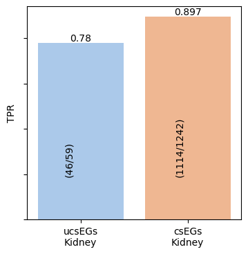
This code can be used to produce Fig 5(B) of the HELP paper by executing
an iteration cycle for both kidney and lung tissues.
At the end, we print the list of ucs_EGs for the tissue.
genes[f'ucsEGs_{tissue}_y']
array(['ACTG1', 'ACTR6', 'ARF4', 'ARPC4', 'CDK6', 'CHMP7', 'COPS3',
       'DCTN3', 'DDX11', 'DDX52', 'EMC3', 'EXOSC1', 'GEMIN7', 'GET3',
       'HGS', 'HTATSF1', 'KIF4A', 'MCM10', 'MDM2', 'METAP2', 'MLST8',
       'NCAPH2', 'NDOR1', 'OXA1L', 'PFN1', 'PIK3C3', 'PPIE', 'PPP1CA',
       'PPP4R2', 'RAB7A', 'RAD1', 'RBM42', 'RBMX2', 'RTEL1', 'SNRPB2',
       'SPTLC1', 'SRSF10', 'TAF1D', 'TMED10', 'TMED2', 'UBA5', 'UBC',
       'UBE2D3', 'USP10', 'VPS52', 'YWHAZ'], dtype=object)